The dplyr package includes several different kind of joining functions which allow you to join dataframes together, when they share a common id variable. My strategy with joins up until now has been to just try them at random and see which one delivers the data output I’m expecting. Not very efficient.

Here I work through the examples in the documentation to see if I can figure out the difference between inner, left, right, and full joins. And then I try out my join skills on a Tidy Tuesday example about formula one.

library(tidyverse)
library(janitor)
library(tidytuesdayR)
library(naniar)

The Band Example

The examples the dplyr documentation are about band members and instruments.

band_members

## # A tibble: 3 × 2
##   name  band   
##   <chr> <chr>  
## 1 Mick  Stones 
## 2 John  Beatles
## 3 Paul  Beatles

OK the band members are Mick, John and Paul…

band_instruments

## # A tibble: 3 × 2
##   name  plays 
##   <chr> <chr> 
## 1 John  guitar
## 2 Paul  bass  
## 3 Keith guitar

… but the instruments data has info about John, Paul and Keith (but not Mick)

left_join()

left join: adds variables from the right table to the left, keeping all rows from the left.

With left_join(), the output looks more like the left table than the right. We have lost information about Keith, who was in the right table (instruments) but not the left.

left <- left_join(band_members, band_instruments, by = "name")

left

## # A tibble: 3 × 3
##   name  band    plays 
##   <chr> <chr>   <chr> 
## 1 Mick  Stones  <NA>  
## 2 John  Beatles guitar
## 3 Paul  Beatles bass

right_join()

right join: adds variables from the left table to the right, keeping all rows from the right.

Now the output looks more like the right table. We have lost information about Mick, who was in the left table (members) but not the right.

right <- right_join(band_members, band_instruments, by = "name")

right

## # A tibble: 3 × 3
##   name  band    plays 
##   <chr> <chr>   <chr> 
## 1 John  Beatles guitar
## 2 Paul  Beatles bass  
## 3 Keith <NA>    guitar

inner_join

inner join- joins right and left, only keeping rows that have complete data.

oh… we lost information about both Mick and Keith.

inner <- inner_join(band_members, band_instruments, by = "name")

inner

## # A tibble: 2 × 3
##   name  band    plays 
##   <chr> <chr>   <chr> 
## 1 John  Beatles guitar
## 2 Paul  Beatles bass

full_join

full join- joins right and left, keeps all rows from both dataframes.

full_join() might be a recipe for lots of NA but you can be sure you aren’t losing anything.

full <- full_join(band_members, band_instruments, by = "name")

full

## # A tibble: 4 × 3
##   name  band    plays 
##   <chr> <chr>   <chr> 
## 1 Mick  Stones  <NA>  
## 2 John  Beatles guitar
## 3 Paul  Beatles bass  
## 4 Keith <NA>    guitar

What about bigger data?

Tidy Tuesday Formula One

This data comes from Tidy Tuesday Week 37 2021 and it is about formula one races.

tt <- tt_load("2021-10-26")

## 
## 	Downloading file 1 of 2: `ultra_rankings.csv`
## 	Downloading file 2 of 2: `race.csv`

rank <- tt[[1]]

race <- tt[[2]]

glimpse(rank)

## Rows: 137,803
## Columns: 8
## $ race_year_id    <dbl> 68140, 68140, 68140, 68140, 68140, 68140, 68140, 68140…
## $ rank            <dbl> 1, 2, 3, 4, 5, 6, 7, 8, 9, 10, 11, 12, 13, NA, NA, NA,…
## $ runner          <chr> "VERHEUL Jasper", "MOULDING JON", "RICHARDSON Phill", …
## $ time            <chr> "26H 35M 25S", "27H 0M 29S", "28H 49M 7S", "30H 53M 37…
## $ age             <dbl> 30, 43, 38, 55, 48, 31, 55, 40, 47, 29, 48, 47, 52, 49…
## $ gender          <chr> "M", "M", "M", "W", "W", "M", "W", "W", "M", "M", "M",…
## $ nationality     <chr> "GBR", "GBR", "GBR", "GBR", "GBR", "GBR", "GBR", "GBR"…
## $ time_in_seconds <dbl> 95725, 97229, 103747, 111217, 117981, 118000, 120601, …

glimpse(race)

## Rows: 1,207
## Columns: 13
## $ race_year_id   <dbl> 68140, 72496, 69855, 67856, 70469, 66887, 67851, 68241,…
## $ event          <chr> "Peak District Ultras", "UTMB®", "Grand Raid des Pyréné…
## $ race           <chr> "Millstone 100", "UTMB®", "Ultra Tour 160", "PERSENK UL…
## $ city           <chr> "Castleton", "Chamonix", "vielle-Aure", "Asenovgrad", "…
## $ country        <chr> "United Kingdom", "France", "France", "Bulgaria", "Turk…
## $ date           <date> 2021-09-03, 2021-08-27, 2021-08-20, 2021-08-20, 2021-0…
## $ start_time     <time> 19:00:00, 17:00:00, 05:00:00, 18:00:00, 18:00:00, 17:0…
## $ participation  <chr> "solo", "Solo", "solo", "solo", "solo", "solo", "solo",…
## $ distance       <dbl> 166.9, 170.7, 167.0, 164.0, 159.9, 159.9, 163.8, 163.9,…
## $ elevation_gain <dbl> 4520, 9930, 9980, 7490, 100, 9850, 5460, 4630, 6410, 31…
## $ elevation_loss <dbl> -4520, -9930, -9980, -7500, -100, -9850, -5460, -4660, …
## $ aid_stations   <dbl> 10, 11, 13, 13, 12, 15, 5, 8, 13, 23, 13, 5, 12, 15, 0,…
## $ participants   <dbl> 150, 2300, 600, 150, 0, 300, 0, 200, 120, 100, 300, 50,…

OK lets say I want to know more about the winners of each race and the race details. Both dataframes have a race_year_id variable which is a good start, but one has many more observations than the other. First step, make the problem smaller. The rank dataframe has 137803 observations but I think am only interested in the winners, so I am going to filter for rank = 1.

winner <- rank %>%
  filter(rank == 1) 

count(winner)

## # A tibble: 1 × 1
##       n
##   <int>
## 1  1237

Now the winner dataframe has 1237 obs and the race data frame has 1207. I wonder whether there are duplicates in the winner dataframe? get_dupes() from the janitor package is useful for determining whether there are repeated rows in your data.

race %>%
  get_dupes(race_year_id)

## No duplicate combinations found of: race_year_id

## # A tibble: 0 × 14
## # … with 14 variables: race_year_id <dbl>, dupe_count <int>, event <chr>,
## #   race <chr>, city <chr>, country <chr>, date <date>, start_time <time>,
## #   participation <chr>, distance <dbl>, elevation_gain <dbl>,
## #   elevation_loss <dbl>, aid_stations <dbl>, participants <dbl>

winner_dups <- winner %>%
  get_dupes(race_year_id)

count(winner_dups)

## # A tibble: 1 × 1
##       n
##   <int>
## 1    71

Looks like each race is represented only once in the race dataframe, but in the winner dataframe there are some races that had 2 winners!

OK to make it simple lets say I’m only interested in the first of those winners. The distinct() function from dplyr will keep just the distinct rows of a dataframe. If you specify just one variable (rather than the whole row) to check, you need to include .keep_all to prevent all the other variables being removed.

winner_distinct <- winner %>%
  distinct(race_year_id, .keep_all = TRUE)

winner_distinct %>%
  get_dupes()

## No variable names specified - using all columns.

## No duplicate combinations found of: race_year_id, rank, runner, time, age, gender, nationality, time_in_seconds

## # A tibble: 0 × 9
## # … with 9 variables: race_year_id <dbl>, rank <dbl>, runner <chr>, time <chr>,
## #   age <dbl>, gender <chr>, nationality <chr>, time_in_seconds <dbl>,
## #   dupe_count <int>

Now that we have 1207 obs in the race dataframe and 1200 in the winner_distinct dataframe lets try joining them. I am going to select just a few variables first so that it is easier to see how the join comes together.

So from race I am interested in race_year_id, distance, and participants. From winner_distinct, I don’t need rank or time, but will leave the rest.

final_race <- race %>%
  select(race_year_id, distance, participants)
         
final_winner <- winner_distinct %>%
  select(-rank, -time)

Lets try joining them…the left dataframe is winners (1200 obs) and the right is race (1207 obs)

left_join()

First left_join()… we end up with 1200 obs, losing the 7 races that aren’t represented in the winners dataframe.

winner_race_left <- left_join(final_winner, final_race)

## Joining, by = "race_year_id"

count(winner_race_left)

## # A tibble: 1 × 1
##       n
##   <int>
## 1  1200

right_join()

Then right_join(), 1207 observations (same as race dataframe) which means that there must be some missing values.

winner_race_right <- right_join(final_winner, final_race)

## Joining, by = "race_year_id"

count(winner_race_right)

## # A tibble: 1 × 1
##       n
##   <int>
## 1  1207

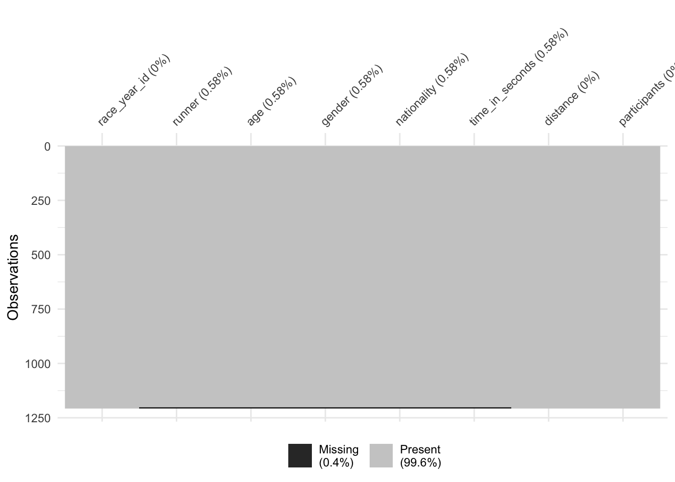
The vis_miss() function from the naniar package is a useful way of seeing where missing values are in your data. Here is looks like there are a small number of observations missing from the winner variables runner:time_in_seconds data.

vis_miss(winner_race_right)

## Warning: `gather_()` was deprecated in tidyr 1.2.0.
## Please use `gather()` instead.
## This warning is displayed once every 8 hours.
## Call `lifecycle::last_lifecycle_warnings()` to see where this warning was generated.

inner_join()

This confusing, inner_join() also results in 1207 obs. I expected it to drop rows where the data wasn’t complete?

winner_race_inner <- right_join(final_winner, final_race, by = "race_year_id")

vis_miss(winner_race_inner)

full_join()

full_join() keeps everything, as expected.

winner_race_full <- right_join(final_winner, final_race)

## Joining, by = "race_year_id"

count(winner_race_full)

## # A tibble: 1 × 1
##       n
##   <int>
## 1  1207

At this point, I am running out of energy to work out why inner_join() is not doing what I thought it was supposed to do, but I am interested in which races have values that aren’t in the winner dataframe. That is where anti_join() comes in…

anti_join()

You need to change the order of the left and right dataframes because you are asking R to find the values in race than AREN’T in winner

winner_race_anti <- anti_join(final_race, final_winner)

## Joining, by = "race_year_id"

winner_race_anti

## # A tibble: 7 × 3
##   race_year_id distance participants
##          <dbl>    <dbl>        <dbl>
## 1        51397     163.           50
## 2        65591     172.           50
## 3        36091     170.           50
## 4        21335     162            50
## 5        26383     168.           15
## 6        21659     160.           50
## 7        10297     165.           80

anti_join() for the win!!